7 Spatiotemporal Segregation Dynamics

Code

%load_ext watermark
%watermark -v -a "author: eli knaap" -d -u -p segregation,libpysal,geopandas,geosnap

Author: author: eli knaap

Last updated: 2024-01-22

Python implementation: CPython
Python version       : 3.11.0
IPython version      : 8.18.1

segregation: 2.5
libpysal   : 4.9.2
geopandas  : 0.14.2
geosnap    : 0.12.1.dev9+g3a1cb0f6de61.d20240110

Some plots in this notebook require hvplot, which is not a standard geosnap dependency

Code

import pandas as pd
import geopandas as gpd
import matplotlib.pyplot as plt
import hvplot.pandas

from segregation import singlegroup, multigroup, dynamics, batch
from geosnap import DataStore
from geosnap import io as gio
from geosnap.analyze import segdyn

Code

from geosnap.visualize import plot_timeseries

Code

datasets = DataStore()

Code

dc = gio.get_acs(datasets, msa_fips='47900', years=[2012, 2016,])
dc21 =  gio.get_acs(datasets, msa_fips='47900', years=[2021])
dc21=dc21.set_crs(dc.crs)
dc = gpd.GeoDataFrame(pd.concat([dc,dc21]))

/Users/knaaptime/Dropbox/projects/geosnap/geosnap/io/constructors.py:188: UserWarning: `constant_dollars` is True, but no `currency_year` was specified. Resorting to max value of 2016
  warn(
/Users/knaaptime/Dropbox/projects/geosnap/geosnap/io/util.py:275: UserWarning: Unable to find local adjustment year for 2021. Attempting from online data
  warn(
/Users/knaaptime/Dropbox/projects/geosnap/geosnap/io/constructors.py:215: UserWarning: Currency columns unavailable at this resolution; not adjusting for inflation
  warn(

Code

dc = dc.to_crs(dc.estimate_utm_crs())

Code

dc.head()

	geoid	n_total_housing_units	n_vacant_housing_units	n_occupied_housing_units	n_owner_occupied_housing_units	n_renter_occupied_housing_units	n_housing_units_multiunit_structures_denom	n_housing_units_multiunit_structures	n_total_housing_units_sample	median_home_value	...	p_hispanic_persons	p_native_persons	p_asian_persons	p_asian_indian_persons	p_edu_college_greater	p_veterans	geometry	year
0	110010001001	776.0	120.0	656.0	245.0	411.0	776.0	375.0	776.0	1.014441e+06	...	12.808642	0.000000	3.395062	3.395062	87.141444	4.938272	MULTIPOLYGON (((320658.461 4309603.540, 320718...	2012
1	110010001002	907.0	110.0	797.0	369.0	428.0	907.0	546.0	907.0	7.830297e+05	...	1.210287	0.000000	3.479576	3.479576	86.875612	5.975794	MULTIPOLYGON (((321636.641 4308861.303, 321646...	2012
2	110010001003	589.0	39.0	550.0	391.0	159.0	589.0	221.0	589.0	1.047112e+06	...	4.755245	5.664336	7.552448	7.552448	97.289448	8.181818	MULTIPOLYGON (((320967.686 4308858.767, 320969...	2012
3	110010001004	552.0	102.0	450.0	256.0	194.0	552.0	166.0	552.0	1.047112e+06	...	1.612903	0.000000	6.854839	6.854839	85.314685	4.334677	MULTIPOLYGON (((320608.256 4307826.451, 321099...	2012
4	110010002011	0.0	0.0	0.0	0.0	0.0	0.0	0.0	0.0	NaN	...	4.442808	0.000000	12.272950	12.272950	49.382716	0.000000	MULTIPOLYGON (((319785.287 4309141.585, 319879...	2012

5 rows × 58 columns

Code

from IPython.display import IFrame

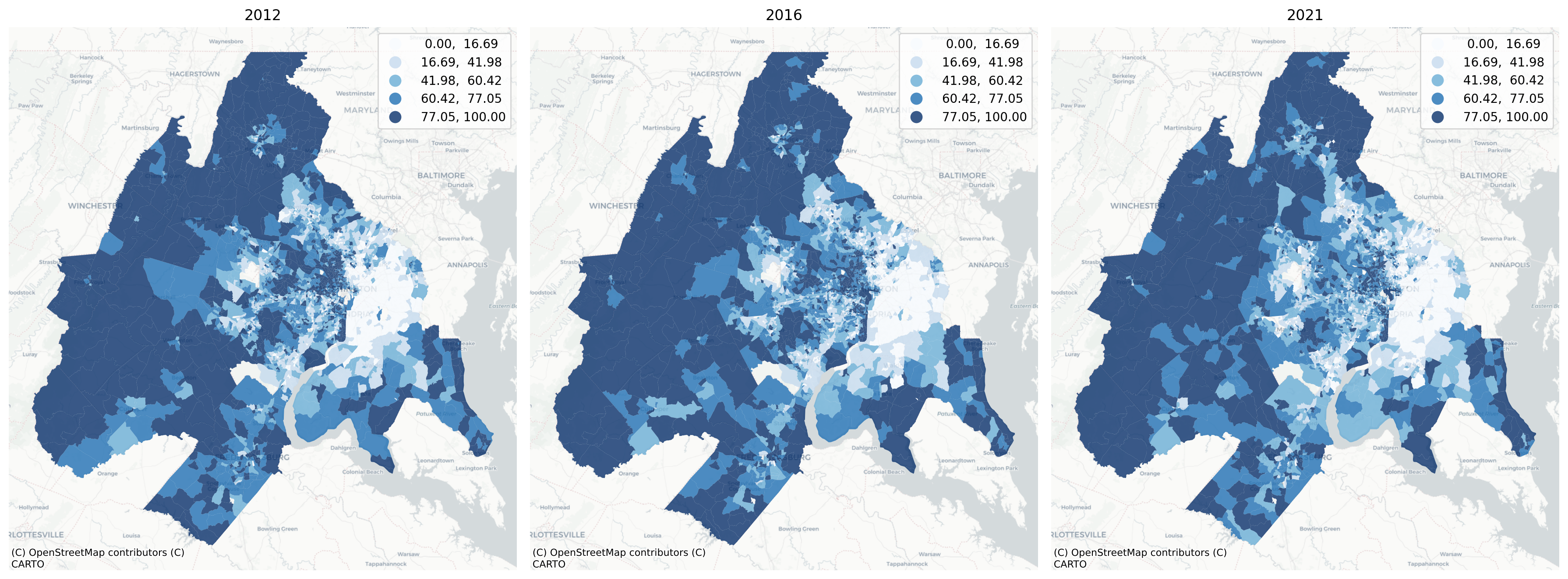
7.1 Racial Segregation over Time

Code

groups = ['n_nonhisp_white_persons', 'n_nonhisp_black_persons', 'n_hispanic_persons', 'n_asian_persons']

Code

plot_timeseries(dc, 'p_nonhisp_white_persons', nrows=1, ncols=3, figsize=(18,10), cmap='Blues', alpha=0.8)
plt.tight_layout()

/Users/knaaptime/Dropbox/projects/geosnap/geosnap/visualize/mapping.py:170: UserWarning: `proplot` is not installed.  Falling back to matplotlib
  warn("`proplot` is not installed.  Falling back to matplotlib")

7.1.1 Temporal Dynamics

7.1.1.1 Multi-Group Indices

Code

multi_by_time = segdyn.multigroup_tempdyn(dc, groups)

Code

multi_by_time

year	2012	2016	2021
Name
GlobalDistortion	191.2887	179.0859	195.9176
MultiDissim	0.5263	0.5138	0.5151
MultiDivergence	0.3845	0.3727	0.3900
MultiDiversity	1.1958	1.2200	1.2499
MultiGini	0.6952	0.6788	0.6816
MultiInfoTheory	0.3215	0.3055	0.3120
MultiNormExposure	0.3315	0.3169	0.3150
MultiRelativeDiversity	0.3196	0.3061	0.3066
MultiSquaredCoefVar	0.2640	0.2579	0.2700
SimpsonsConcentration	0.3503	0.3375	0.3212
SimpsonsInteraction	0.6497	0.6625	0.6788

Code

multi_by_time.T.plot()

<Axes: xlabel='year'>

Code

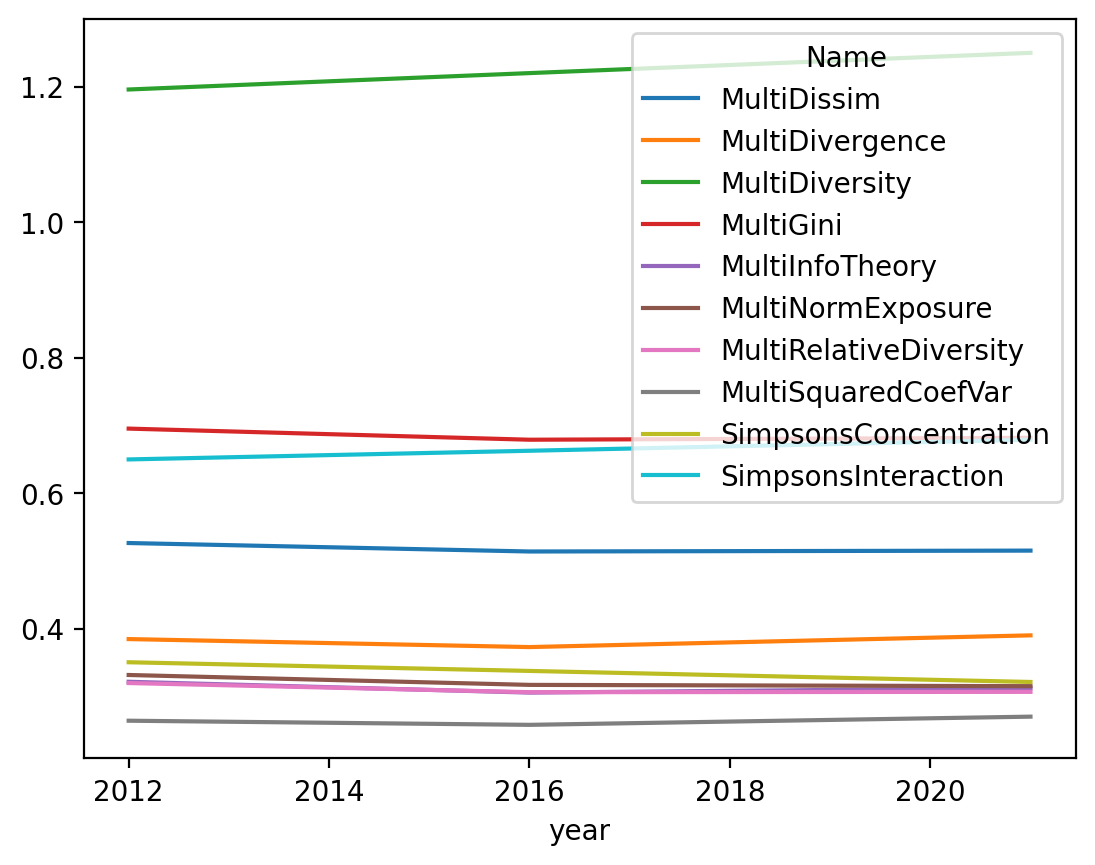
# removing the GlobalDistortion coef lets us see what's happening with the rest of the indices
multi_by_time.iloc[1:].T.plot()

<Axes: xlabel='year'>

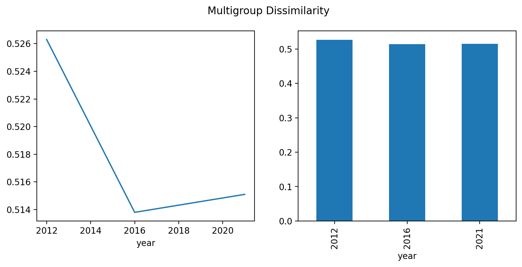
Most indices are changing little over time, but most have followed the same trend with a mild drop in 2016 prior to a slight increase in the latest available data

Code

fig, axs = plt.subplots(1,2, figsize=(10,4))

multi_by_time.loc['MultiDissim'].plot(ax=axs[0])
multi_by_time.loc['MultiDissim'].plot(kind='bar', ax=axs[1])

fig.suptitle("Multigroup Dissimilarity")

Text(0.5, 0.98, 'Multigroup Dissimilarity')

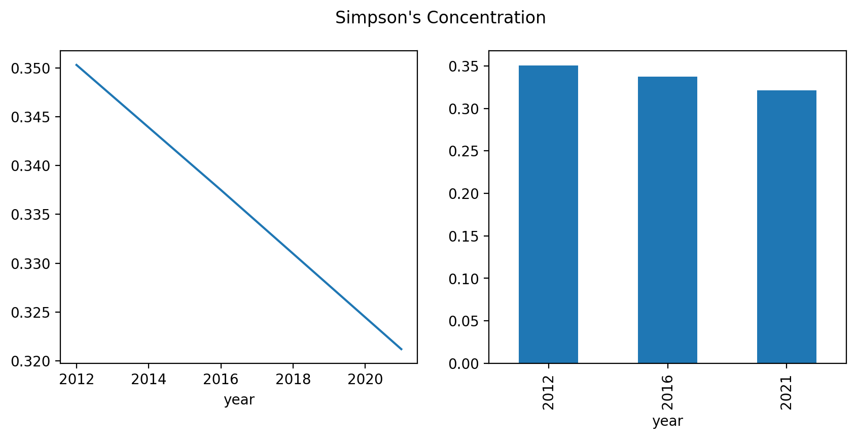
One that isn’t, is SimpsonsConcentration, which is increasing over time. Another index that bucks the trend is SimpsonsInteraction, which is decreasing over time (corresponding with an increse in segregation). The divergence between indices tells us that segregation may be changing in different ways across its different dimensions.

Code

fig, axs = plt.subplots(1,2, figsize=(10,4))

multi_by_time.loc['SimpsonsConcentration'].plot(ax=axs[0])
multi_by_time.loc['SimpsonsConcentration'].plot(kind='bar', ax=axs[1])

fig.suptitle("Simpson's Concentration")

Text(0.5, 0.98, "Simpson's Concentration")

7.1.1.2 Single-Group Indices

Code

from geosnap.analyze.segdyn import singlegroup_tempdyn

Code

singlegroup_tempdyn?

Signature:
singlegroup_tempdyn(
    gdf,
    group_pop_var=None,
    total_pop_var=None,
    time_index='year',
    n_jobs=-1,
    backend='loky',
    **index_kwargs,
)
Docstring:
Batch compute singlegroup segregation indices for each time period in parallel.
Parameters
----------
gdf : geopandas.GeoDataFrame
    geodataframe formatted as a long-form timeseries
group_pop_var : str
    name of column on gdf containing population counts for the group of interest
total_pop_var : str
    name of column on gdf containing total population counts for the unit
time_index : str
    column on the dataframe that denotes unique time periods, by default "year"
n_jobs : int, optional
    number of cores to use for computation. If -1, all available cores will be
    used, by default -1
backend : str, optional
    computation backend passed to joblib. One of {'multiprocessing', 'loky',
    'threading'}, by default "loky"
Returns
-------
geopandas.GeoDataFrame
    dataframe with unique segregation indices as rows and estimates for each
    time period as columns
File:      ~/Dropbox/projects/geosnap/geosnap/analyze/segdyn.py
Type:      function

Code

dc['blackwhite'] = dc.n_nonhisp_black_persons + dc.n_nonhisp_white_persons

Code

segs_single = segdyn.singlegroup_tempdyn(dc, group_pop_var='n_nonhisp_black_persons', total_pop_var='blackwhite' )

Gini:  52%|█████▏    | 14/27 [00:19<00:19,  1.51s/it]                    OMP: Info #276: omp_set_nested routine deprecated, please use omp_set_max_active_levels instead.
ModifiedDissim:  67%|██████▋   | 18/27 [00:20<00:11,  1.29s/it]OMP: Info #276: omp_set_nested routine deprecated, please use omp_set_max_active_levels instead.
ModifiedGini:  70%|███████   | 19/27 [00:22<00:06,  1.27it/s]            OMP: Info #276: omp_set_nested routine deprecated, please use omp_set_max_active_levels instead.
SpatialProximity: 100%|██████████| 27/27 [00:52<00:00,  1.96s/it]      
SpatialProximity: 100%|██████████| 27/27 [00:53<00:00,  1.99s/it]
SpatialProximity: 100%|██████████| 27/27 [01:02<00:00,  2.33s/it]

Code

segs_single

year	2012	2016	2021
Name
AbsoluteCentralization	0.6945	0.6938	0.6804
AbsoluteClustering	0.3263	0.3326	0.3613
AbsoluteConcentration	0.8278	0.8284	0.8270
Atkinson	0.6294	0.6069	0.6106
BiasCorrectedDissim	0.6523	0.6443	0.6463
BoundarySpatialDissim	0.5239	0.5191	0.4999
ConProf	0.6069	0.6020	0.6068
CorrelationR	0.5192	0.5065	0.5097
Delta	0.7937	0.7921	0.7920
DensityCorrectedDissim	0.5064	0.4942	0.5153
Dissim	0.6526	0.6446	0.6466
DistanceDecayInteraction	0.4776	0.4797	0.4707
DistanceDecayIsolation	0.5349	0.5366	0.5523
Entropy	0.4665	0.4511	0.4538
Gini	0.8248	0.8137	0.8164
Interaction	0.3174	0.3227	0.3144
Isolation	0.6826	0.6773	0.6856
MinMax	0.7898	0.7839	0.7854
ModifiedDissim	0.6441	0.6361	0.6377
ModifiedGini	0.8186	0.8072	0.8098
PARDissim	0.6379	0.6303	0.6327
RelativeCentralization	-0.0193	-0.0258	-0.0424
RelativeClustering	0.7093	0.7241	0.7556
RelativeConcentration	0.6029	0.6142	0.6299
SpatialDissim	0.5171	0.5121	0.4943
SpatialProxProf	0.5772	0.5896	0.6116
SpatialProximity	1.2668	1.2650	1.2801

Code

segs_single.T.hvplot(height=600)

https://www.jstor.org/stable/2579183

Code

IFrame('https://www.jstor.org/stable/2579183', height=600, width=800)

Code

(segs_single.T[['Gini', 'Entropy', 'Dissim', 'Atkinson']].hvplot(title='Evenness Dimension', width=380, height=400).opts(legend_position='bottom', show_grid=True) +
segs_single.T[['AbsoluteConcentration', 'RelativeConcentration' , 'Delta']].hvplot(title='Concentration Dimension', width=380, height=400).opts(legend_position='bottom', show_grid=True) +
segs_single.T[['AbsoluteClustering', 'Isolation', 'CorrelationR', 'Interaction', 'SpatialProxProf']].hvplot(title='Exposure/Clustering Dimension', width=380, height=400).opts(legend_position='bottom', show_grid=True))

Code

segs_single.T[['AbsoluteClustering', 'Isolation', 'SpatialProxProf', 'Interaction']].pct_change(periods=5) # we should only compare non-overlapping intervals

Name	AbsoluteClustering	Isolation	SpatialProxProf	Interaction
year
2012	NaN	NaN	NaN	NaN
2016	NaN	NaN	NaN	NaN
2021	NaN	NaN	NaN	NaN

Between the sampling periods 2008-2012 and 2013-2017: - the isolation index increased by 5.2% - the absolute clustering index increased by 12.4%.
- the spatial proximity profile increased by 17.6%

Between the sampling periods 2009-2013 and 2014-2018: - the isolation index increased by 7.9% - the absolute clustering index increased by 18.2% - the spatial proximity profile increased by 21.9%

7.2 Space-Time Dynamics

Code

from segregation.singlegroup import Entropy

Code

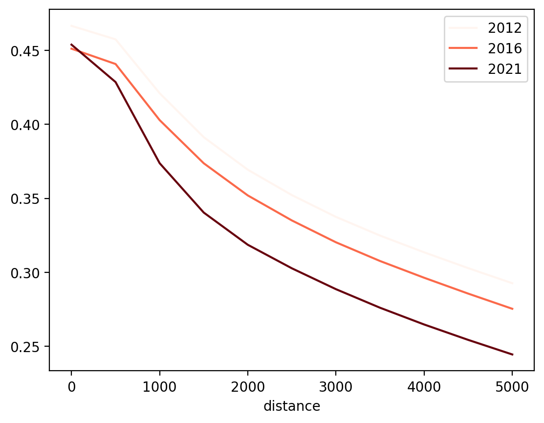
d = segdyn.spacetime_dyn(dc, singlegroup.Entropy, group_pop_var='n_nonhisp_black_persons', total_pop_var='blackwhite', distances=list(range(500,5500,500)))

Code

d.plot(cmap='Reds')

<Axes: xlabel='distance'>

Entropy is falling the fastest at large scales (the gap is wider on the right-hand side of the graph than the left-hand side)

Code

iso = segdyn.spacetime_dyn(dc, singlegroup.Isolation, group_pop_var='n_nonhisp_black_persons', total_pop_var='blackwhite', distances=list(range(500,5500,500)))

Code

iso.plot(cmap='Reds')

<Axes: xlabel='distance'>

Isolation is growing the fastest at large scales (the gap is wider with larger distances on the right). Isolation is actually growing at the smallest scale

Code

from geosnap.visualize import animate_timeseries

Code

animate_timeseries(dc, 'p_nonhisp_black_persons', filename='images/dc_black_pop_change.gif', fps=1.5)

<Figure size 2000x2000 with 0 Axes>

<Figure size 2000x2000 with 0 Axes>

<Figure size 2000x2000 with 0 Axes>

<Figure size 1000x1000 with 0 Axes>

7.3 Using geosnap as a Dashboard Engine

The Python dashboarding ecosystem is evolving quickly, so we won’t opine on which platform or toolset is best. But if you have a personal favorite, geosnap is performant to power an urban analytics dashboard on-the-fly. The example below wraps a simple streamlit interface around the workflow above that lets us explore every metro region quickly

example: https://github.com/knaaptime/incseg_app