Author: eli knaap

Last updated: 2024-01-23

Python implementation: CPython
Python version       : 3.11.0
IPython version      : 8.18.1

geopandas: 0.14.2
geosnap  : 0.12.1.dev9+g3a1cb0f6de61.d20240110
8.1 Visualizing the 20-Minute Neighborhood
As a package focused on “neighborhoods”, much of the functionality in geosnap is organized around the concept of ‘endogenous’ neighborhoods. That is, it takes a classical perspective on neighborhood formation: a ‘neighborhood’ is defined loosely by its social composition, and the dynamics of residential mobility mean that these neighborhoods can grow, shrink, or transition entirely.
But two alternative concepts of “neighborhood” are also worth considering. The first, posited by social scientists, is that each person or household can be conceptialized as residing in its own neighborhood which extends outward from the person’s household until some threshold distance. This neighborhood represents the boundary inside which we might expect some social interaction to occur with one’s ‘neighbors’. The second is a normative concept advocated by architects, urban designers, and planners (arguably still the goal for new urbanists): that a neighborhood is a discrete pocket of infrastructure organized as a small, self-contained economic unit. A common shorthand today is the 20 minute neighborhood.
The difference between these two perspectives is really what defines the origin of the neighborhood (the ‘town center’ or the person’s home), and whether ‘neighborhood’ is universal to all neighbors or unique for each resident. Both of them rely abstractly on the concept of an isochrone: the set of destinations accessible within a specified travel budget. Defining an isochrone is a network routing problem, but its spatial representation is usually given as a polygon that covers the set of locations. That polygon is also sometimes called a walkshed (or *travel shed, depending on the particular mode). For the person at the center of the isochrone, whose “neighborhood” the isochrone represents, the polygon is sometimes conceptualized as an “egohood” or “bespoke neighborhood”.
The trouble with generating isochrones is twofold. First, they are computationally intensive to create. You need to know the shortest path from an origin to all other possible destinations inside the travel threshold, and depending on the density of the network, this can scale masssively. Second, they are not straightforward to present cartographically/visually. The set of destinations reachable within the threshold is technically a set of points. If you’re constrained to a network, then we can usually assume that you also have access to potential locations between discrete destinations. For example if you’re walking along the sidewalk, you can stop at any house along the block until you reach your threshold distance. But sometimes that’s not the case. If you walk to a subway station, you can stop anywhere along the walk–until you get into the subway, then you are stuck traveling in one direction until you reach another station, then you get freedom of mobility again.
The latter case is particularly difficult to represent because it doesnt create a “valid” polygon… there’s a single polygon in the pre-transit zone, then the “accessible zone” collapses to a line (or nothing at all?) before opening back up into a polygon again. Like a barbell. If you take the simple route and just draw a convex hull around the accessible destinations, it will fail to collapse along the line, giving the false impression of much more ‘access’ than is realistic.
But then again, sometimes these off-network spaces are actually traversable. If two network nodes inside the travel threshold are separated by a park, then you can just walk through the park and that should be included in the visualization. If they are separated by a harbor or a mountain, you definitely can’t walk through (ok, maybe you could get through, but not without sacrificing a bit of speed at the very least).
To handle these issues, the isochrones implemented in geosnap take a straightforward approach, achieving a good balance between accuracy and speed. Specifically, we tackle the problem in two stages: first, we use pandana to generate the set nodes accessible from [a set of] destination[s]. Then we wrap an alpha shape around those destinations to create a tightly-fitted polygon. The alpha shape algorithm implemented in libpysal is also blazing fast, so the approach has worked quite well in all of our applications
Code
from geosnap.analyze import isochrones_from_id, isochrones_from_gdf, pdna_to_adj from geosnap.io import get_acsfrom geosnap import DataStore
Code
import pandana as pdnaimport geopandas as gpd
Code
datasets = DataStore()
To generate a routable network, use pandana or urbanaccess. Alternatively, you can download one of the metropolitan-scale pedestrian networks for the U.S. from geosnap’s quilt bucket. The files are named for each CBSA fips code and extend 8km beyond the metro region’s borders to help mitigate edge effects. Here, we’ll use the quilt version from the San Diego region.
/Users/knaaptime/Dropbox/projects/geosnap/geosnap/io/constructors.py:215: UserWarning: Currency columns unavailable at this resolution; not adjusting for inflation
  warn(
Code
import osifnot os.path.exists('41740.h5'):import quilt3 as q3 b = q3.Bucket("s3://spatial-ucr") b.fetch("osm/metro_networks_8k/41740.h5", "./41740.h5")sd_network = pdna.Network.from_hdf5("41740.h5")
Generating contraction hierarchies with 10 threads.
Setting CH node vector of size 332554
Setting CH edge vector of size 522484
Range graph removed 143094 edges of 1044968
. 10% . 20% . 30% . 40% . 50% . 60% . 70% . 80% . 90% . 100%
To generate a travel isochrone, we have to specify an origin node on the network. For demonstration purposes, we can randomly select an origin from the network’s nodes_df dataframe (or choose a pre-selected example). To get the nodes for a specific set of origins, you can use pandana’s get_node_ids function
Nike, er… this study says that the average person walks about a mile in 20 minutes, so we can define the 20-minute neighborhood for a given household as the 1-mile walkshed from that house. To simplify the computation a little, we say that each house “exists” at it’s nearest intersection
(this is the abstraction pandana typically uses to simplify the problem when using data from OpenStreetMap. There’s nothing prohibiting you from creating an even more realistic version with nodes for each residence, as long as you’re comfortable creating the Network)
/Users/knaaptime/Dropbox/projects/geosnap/geosnap/analyze/network.py:34: UserWarning: Geometry is in a geographic CRS. Results from 'centroid' are likely incorrect. Use 'GeoSeries.to_crs()' to re-project geometries to a projected CRS before this operation.

  node_ids = network.get_node_ids(origins.centroid.x, origins.centroid.y).astype(int)
Code
adj
origin
destination
cost
0
060730001001
060730001001
0.000000
136
060730001001
060730001002
987.565979
197
060730001001
060730002011
1221.943970
240
060730001001
060730002022
1465.890991
280
060730001002
060730001002
0.000000
...
...
...
...
1036301
060730166072
060730166071
1596.958008
1036304
060730166073
060730166073
0.000000
1036489
060730166073
060730166071
932.747009
1036512
060730166073
060730166072
982.960022
1036608
060730166073
060730166101
1229.456055
11391 rows × 3 columns
Code
%%timeiso = isochrones_from_id(example_origin, sd_network, threshold=1600 ) # network is expressed in meters
/Users/knaaptime/Dropbox/projects/geosnap/geosnap/analyze/network.py:34: UserWarning: Geometry is in a geographic CRS. Results from 'centroid' are likely incorrect. Use 'GeoSeries.to_crs()' to re-project geometries to a projected CRS before this operation.

  node_ids = network.get_node_ids(origins.centroid.x, origins.centroid.y).astype(int)
CPU times: user 925 ms, sys: 44.1 ms, total: 969 ms
Wall time: 979 ms
Code
iso.explore()
Make this Notebook Trusted to load map: File -> Trust Notebook
We can also look at how the isochrone or bespoke neighborhood changes size and shape as we consider alternative travel thresholds. Because of the underlying network configuration, changing the threshold often results in some areas of the “neighborhood” changing more than others
/Users/knaaptime/Dropbox/projects/geosnap/geosnap/analyze/network.py:34: UserWarning: Geometry is in a geographic CRS. Results from 'centroid' are likely incorrect. Use 'GeoSeries.to_crs()' to re-project geometries to a projected CRS before this operation.

  node_ids = network.get_node_ids(origins.centroid.x, origins.centroid.y).astype(int)
CPU times: user 593 ms, sys: 18.9 ms, total: 612 ms
Wall time: 644 ms
Make this Notebook Trusted to load map: File -> Trust Notebook
In this example it’s easy to see how the road network topology makes it easier to travel in some directions more than others. Greenspace squeezes the western portion of the 1600m (20 min) isochrone into a horizontal pattern along Calle del Cerro, but the 2400m (30 minute) isochrone opens north-south tavel again along Avienda Pico, providing access to two other pockets of development, including San Clemente High School
We can also compare the network-based isochrone to the as-the-crow-flies approximation given by a euclidean buffer. If we didn’t have access to network data, this would be our best estimate of the shape and extent of the 20-minute neighborhood.
# convert the node into a Point and buffer it 1600mexample_point = gpd.GeoDataFrame(sd_network.nodes_df.loc[example_origin]).T.set_geometry('geometry')example_point = example_point.set_crs(4326)planar_iso = example_point.to_crs(example_point.estimate_utm_crs()).buffer(1600)
Code
# plot the buffer and isochrone on the same mapm = planar_iso.to_crs(4326).explore()iso.explore(m=m)
Make this Notebook Trusted to load map: File -> Trust Notebook
Obviously from this depiction, network-constrained travel is very different from a euclidean approximation. That’s especially true in places with irregular networks or topography considerations (like much of California)
8.2 Isochrones for Specified Locations
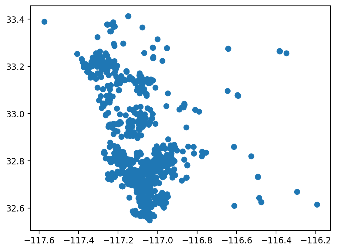
the isochrones function calculates several isochrones simultaneously, given a set of input destinations. For example we could look at the 20-minute neighborhood for schools in San Diego county.
Code
from geosnap.io import get_nces
Code
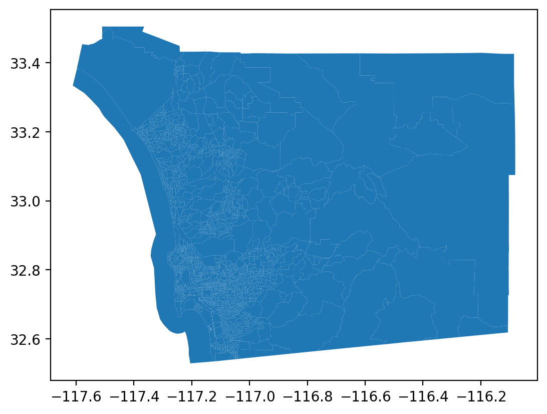
# same as county fips 06073 in this case, but use metro fips for consistency with networksd = get_acs(datasets, msa_fips='41740', level='bg', years=[2019])
# randomly sample 25 schools and compute their walkshedsschool_neighborhoods = isochrones_from_gdf(origins=sd_schools.sample(25), network=sd_network, threshold=1600,)
/Users/knaaptime/Dropbox/projects/geosnap/geosnap/analyze/network.py:140: UserWarning: Geometry is in a geographic CRS. Results from 'centroid' are likely incorrect. Use 'GeoSeries.to_crs()' to re-project geometries to a projected CRS before this operation.

  node_ids = network.get_node_ids(origins.centroid.x, origins.centroid.y).astype(int)
/Users/knaaptime/Dropbox/projects/geosnap/geosnap/analyze/network.py:34: UserWarning: Geometry is in a geographic CRS. Results from 'centroid' are likely incorrect. Use 'GeoSeries.to_crs()' to re-project geometries to a projected CRS before this operation.

  node_ids = network.get_node_ids(origins.centroid.x, origins.centroid.y).astype(int)
Code
school_neighborhoods
geometry
distance
origin
13662
POLYGON ((-117.14646 32.71848, -117.14598 32.7...
1600
13745
POLYGON ((-117.15657 32.72294, -117.15569 32.7...
1600
6045
POLYGON ((-117.02136 33.27643, -117.02352 33.2...
1600
14426
POLYGON ((-117.00264 32.84421, -117.00343 32.8...
1600
14132
POLYGON ((-117.16720 33.13873, -117.16856 33.1...
1600
13672
POLYGON ((-117.17622 32.76935, -117.17913 32.7...
1600
9634
POLYGON ((-117.01525 32.71985, -117.01392 32.7...
1600
11677
POLYGON ((-116.19684 32.61392, -116.19287 32.6...
1600
5895
POLYGON ((-116.64411 33.27421, -116.64491 33.2...
1600
14651
POLYGON ((-117.11173 32.58916, -117.10999 32.5...
1600
13639
POLYGON ((-117.10254 32.91271, -117.10192 32.9...
1600
7204
POLYGON ((-116.91462 32.79367, -116.91456 32.7...
1600
9129
POLYGON ((-116.93932 32.79346, -116.94135 32.7...
1600
13604
POLYGON ((-117.18463 32.83899, -117.18164 32.8...
1600
15758
POLYGON ((-117.17343 32.71976, -117.17318 32.7...
1600
8558
POLYGON ((-117.25935 33.37671, -117.25949 33.3...
1600
8426
POLYGON ((-117.03368 33.13773, -117.03259 33.1...
1600
7623
POLYGON ((-117.00010 32.62969, -116.99944 32.6...
1600
13560
POLYGON ((-117.09858 32.68953, -117.09757 32.6...
1600
14655
POLYGON ((-117.11923 32.56924, -117.11969 32.5...
1600
12859
POLYGON ((-117.06596 32.98104, -117.06585 32.9...
1600
14847
POLYGON ((-117.06425 32.61504, -117.06297 32.6...
1600
13561
POLYGON ((-117.21433 32.80365, -117.21415 32.8...
1600
13632
POLYGON ((-117.08379 32.74163, -117.08414 32.7...
1600
13550
POLYGON ((-117.09290 32.83455, -117.09509 32.8...
1600
Code
school_neighborhoods.explore()
Make this Notebook Trusted to load map: File -> Trust Notebook
If we adopt the “neighborhood unit” perspective, it might be reasonable to put a school at the center of the neighborhood, as it would provide equitable access to all residents. In that case, these are your neighborhoods
8.3 Extensions
One nice thing about this implementation is that it’s indifferent to the structure of the input network. It could be pedestrian-based (which is the most common), but you could also use urbanaccess to create a multimodel network by combining OSM and GTFS data. For this reason, the isochrone function provided here can be much more useful than commercially-provided web services like mapbox, first because all the computation happens locally (so no paywall, and no unwanted data collection) and second because the researcher has full control over how the network is structured. This allows you to do the kinds of analyses common in actual transportation modeling and planning–like adding a new transit line, a new lane in the freeway, or a new toll road, and see how the accessibility surface responds (and how the location choices of households and businesses will reallocate given this new geography).
Running the above functions on that multimodal network would give a good sense of “baseline” accessibility in a study region. An interested researcher could then make some changes to the GTFS network, say, by increasing bus frequency along a given corridor, then create another combined network and compare results. Who would benefit from such a change, and what might be the net costs?
And thus, the seeds of open and reproduciblescenario planning have been sown :)